Background - Generative Models v.s. Discriminative Models

In machine learning, supervised learning can be divided into two kinds: Generative and discriminative. Generative models can generate new data instances by capturing the joint probability $p(X, Y)$, while discriminative models discriminate between different kinds of data instances by capturing the conditional probability $p(Y| X)$.

Say that we want to solve a classification problem ($C_1, C_2, \dots, C_I$), for a new sample $x$, we want to predict its category by calculating the maximum conditional probability $p(y | x)$.

Generative Models

Generative Models have to model the distribution throughout the data space. The key point is to first assume the probability distribution of the data; then obtain statistical value for this distribution; finally calculate the probability of a certain sample for different classes and get the prediction by the Bayesian formula.

Usually we suppose the data distribution is Gaussian distribution because it’s easy to calculate and is abundant in the natural world. For $C_i$, the mean $\mu_i$ and variance $\Sigma_i$ of its Gaussian distributions are computed by certain methods (like the Maximum Likelihood Estimate). After having class data distributions, the probability that a sample $x$ belongs to class $C_i$ is:

\[P\left(x | C_i\right) = N(\mu_i, \Sigma_i) =\frac{1}{(2 \pi)^{D / 2}} \frac{1}{\left|\Sigma_i\right|^{1 / 2}} \exp \left\{-\frac{1}{2}\left(x-\mu_i\right)^T \Sigma_i^{-1}\left(x-\mu_i\right)\right\},\]

where $D$ is the dimension of $x$. Now we have $P(C_i)$ and $P(x|C_i)$, according to the Bayesian formula, the probability that $x$ belongs to class $C_i$ can be computed as:

\[P(C_i|x) = \frac{P(x, C_i)}{P(x)} = \frac{P(x|C_i)P(C_i)}{\Sigma_{j=1}^{I} P(x|C_j)P(C_j)}\]

Finally, choose the one with maximum probability as the predicted class for the given sample $x$.

Discriminative Models

Discriminative models directly solve the conditional probability $P(C_i|x)$ by building a network. Then train this network to get the proper value for model weight. They cannot reflect the characteristics of the training data themselves, and only tell us the classification information, so they are more limited.

What are diffusion models?

(Most of the content in this part comes from [1], if you want to see more detailed reasoning, please check the original blog.)

Diffusion models are one kind of Generative Model (others include GAN, VAE), and define a Markov chain that slowly adds Gaussian Noise into data (Forward Diffusion Process), and then learn to remove these noises and reconstruct the sample data (Reverse Denoising Process). The main difference between diffusion and other generative models is that its latent code is the same dimension as the original input. In the following parts, diffusion models will be explained based on DDPM [2].

Forward Diffusion Process

The Forward Diffusion Process will translate a real data point $x_0 \sim q(x)$ to a Gaussian Distribution by adding a small amount of Gaussian noise step by step (in $T$ steps). This produces a series of noisy samples $x_1, x_2, \dots, x_t$. The data $x_t$ has lesser information when the time step $t$ becomes larger, and with very small step size and total steps $T \rightarrow \infty$, the final latent code $x_T$ is equivalent to an isotropic Gaussian distribution $\mathcal{N}(0,1)$.

\[\begin{gather} q(\mathbf{x}_t \vert \mathbf{x}_{t-1}) = \mathcal{N}(\mathbf{x}_t; \sqrt{1 - \beta_t} \mathbf{x }_{t-1}, \beta_t\mathbf{I}) \quad q(\mathbf{x}_{1:T} \vert \mathbf{x}_0) = \prod^T_{t=1} q(\mathbf{x}_t \vert \mathbf{x}_{t-1}) \\ \text{sch} = \{ \beta_t \in (0,1)\}^T_{t=1} \end{gather}\]

The step sizes are controlled by a variance schedule $\text{sch}$, and in practice, $\beta_t$ increases as $t$ increases. The above process can be illustrated as the following figure:

There are two crucial characteristics of the forward process, arbitrary time-step sampling and the reparameterization trick, that help the implementation of diffusion models a lot.

#1 Reparameterization Trick

Because sampling from a distribution is a stochastic process, we cannot backpropagate the gradient. Here, as other works (e.g. VAE) did, the reparameterization trick is used to make it trainable. For example, a sample $\mathbf{z}$ sampled from a (Gaussian) distribution $q_\phi(\mathbf{z}\vert\mathbf{x})$ can be represented by $\boldsymbol{\mu}$ and $\boldsymbol{\sigma}$, which can be learned by a neural network, and the stochasticity is performed by an auxiliary independent random variable $\boldsymbol{\epsilon}$. After the reparameterization, $\mathbf{z}$ still satisfies a Gaussian distribution with mean $\boldsymbol{\mu}$ and variance $\boldsymbol{\sigma}^2$.

\[\begin{aligned} \mathbf{z} &\sim q_\phi(\mathbf{z}\vert\mathbf{x}^{(i)}) = \mathcal{N}(\mathbf{z}; \boldsymbol{\mu}^{(i)}, \boldsymbol{\sigma}^{2(i)}\boldsymbol{I}) & \\ \mathbf{z} &= \boldsymbol{\mu} + \boldsymbol{\sigma} \odot \boldsymbol{\epsilon} \text{, where } \boldsymbol{\epsilon} \sim \mathcal{N}(0, \boldsymbol{I}) \end{aligned}\]

#2 Arbitrary Time-step Sampling

Given the initial input $x_0$ and $\beta$, we can get the noised data $x_t$ at an arbitrary time. Let $\alpha_t = 1 - \beta_t$ and $\bar{\alpha}t = \prod{i=1}^t \alpha_i$, using the reparameterization trick, we can get:

\[\begin{array}{rlr} \mathbf{x}_t & =\sqrt{\alpha_t} \mathbf{x}_{t-1}+\sqrt{1-\alpha_t} \boldsymbol{\epsilon}_{t-1} ; \text { where } \boldsymbol{\epsilon}_{t-1}, \boldsymbol{\epsilon}_{t-2}, \cdots \sim \mathcal{N}(\mathbf{0}, \mathbf{I}) \\ & =\sqrt{\alpha_t} (\sqrt{\alpha_{t-1}} \mathbf{x}_{t-2} + \sqrt{1-\alpha_{t-1}} \boldsymbol{\epsilon}_{t-2}) +\sqrt{1-\alpha_t} \boldsymbol{\epsilon}_{t-1} \\ & =\sqrt{\alpha_t \alpha_{t-1}} \mathbf{x}_{t-2} + \color{#E0115F}(\sqrt{\alpha_t(1-\alpha_{t-1})} \boldsymbol{\epsilon}_{t-2} + \sqrt{1-\alpha_t}\boldsymbol{\epsilon}_{t-1}) \\ & =\sqrt{\alpha_t \alpha_{t-1}} \mathbf{x}_{t-2}+\sqrt{1-\alpha_t \alpha_{t-1}} \overline{\boldsymbol{\epsilon}}_{t-2} ; \text { where } \overline{\boldsymbol{\epsilon}}_{t-2} \sim \mathcal{N}(0, I) \text { merges two Gaussians} \\ & =\ldots \\ & =\sqrt{\bar{\alpha}_t} \mathbf{x}_0+\sqrt{1-\bar{\alpha}_t} \boldsymbol{\epsilon}; \text{ where } \bar{\alpha}_t = \prod_{i=1}^t \alpha_i \\ q\left(\mathbf{x}_t \mid \mathbf{x}_0\right) & =\mathcal{N}\left(\mathbf{x}_t ; \sqrt{\bar{\alpha}_t} \mathbf{x}_0,\left(1-\bar{\alpha}_t\right) \mathbf{I}\right) \end{array}\]

Because of the independent Gaussian distribution additivity ($\mathcal{N}\left(0, \sigma_{1}^{2} \mathbf{I}\right)+\mathcal{N}\left(0, \sigma_{2}^{2} \mathbf{I}\right) \sim \mathcal{N}\left(0,\left(\sigma_{1}^{2}+\sigma_{2}^{2}\right) \mathbf{I}\right)$), the pink part in the above formula can be transferred to:

\[\begin{aligned} \sqrt{a_{t}\left(1-\alpha_{t-1}\right)} z_{2} &\sim \mathcal{N}\left(0, a_{t}\left(1-\alpha_{t-1}\right) \mathbf{I}\right) \\ \sqrt{1-\alpha_{t}} z_{1} &\sim \mathcal{N}\left(0,\left(1-\alpha_{t}\right) \mathbf{I}\right) \\ \sqrt{a_{t}\left(1-\alpha_{t-1}\right)} z_{2}+\sqrt{1-\alpha_{t}} z_{1} &\sim \mathcal{N}\left(0,\left[\alpha_{t}\left(1-\alpha_{t-1}\right)+\left(1-\alpha_{t}\right)\right] \mathbf{I}\right) \\ &=\mathcal{N}\left(0,\left(1-\alpha_{t} \alpha_{t-1}\right) \mathbf{I}\right) . \end{aligned}\]

Usually, we use a larger update step when the sample gets noisier, so $\beta_1 < \beta_2 < \dots < \beta_T$ and when $T \rightarrow \infty, x_{T} \sim \mathcal{N}(0, \mathbf{I})$.

Reverse Denoising Process

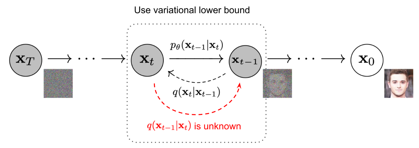
The foward process adds noises to the data gradually, and if we can denoise it by a reverse distrubution $q(x_{t-1} | x_t)$ from a Gaussian noise input $x_T \sim \mathcal{N}(0, \mathbf{I})$, we can generate images. It has been proved that if $q(x_{t} | x_{t-1})$ satisfies the Gaussian distrubution and $\beta_{t}$ is small enough, $q(x_{t-1} | x_t)$ is also a Gaussian distribution. However, we can’t estimate $q(x_{t-1} | x_t)$ because it needs the information of the whole dataset (knowledge of the entire data distribution). Therefore, a model $p_\theta$ (usually is U-Net w/ attention) is learned to approximate these conditional probabilities.

\[\begin{aligned} p_{\theta}\left(X_{0: T}\right) &=p\left(x_{T}\right) \prod_{t=1}^{T} p_{\theta}\left(x_{t-1} \mid x_{t}\right), \\ p_{\theta}\left(x_{t-1} \mid x_{t}\right) &=\mathcal{N}\left(x_{t-1} ; \mu_{\theta}\left(x_{t}, t\right), \Sigma_{\theta}\left(x_{t}, t\right)\right), \end{aligned}\]

where $p\left(x_{T}\right) = \mathcal{N}(0, \mathbf{I})$, $p_{\theta}\left(x_{t-1} \mid x_{t}\right)$ is parameterized Gaussian distribution, whose mean $mu_{\theta}$ and variance $\Sigma_{\theta}$ are provided by trained network. Although the distribution $q(x_{t-1} | x_t)$ is not directly tractable, the posterior distribution conditioned on $x_0$ is tractable. According to Bayes’ rule:

\[\begin{aligned} q\left(\mathbf{x}_{t-1} \mid \mathbf{x}_{t}, \mathbf{x}_{0}\right) &=q\left(\mathbf{x}_{t} \mid \mathbf{x}_{t-1}, \mathbf{x}_{0}\right) \frac{q\left(\mathbf{x}_{t-1} \mid \mathbf{x}_{0}\right)}{q\left(\mathbf{x}_{t} \mid \mathbf{x}_{0}\right)} \\ \end{aligned}\]

Because the process is a Markov Chain, and the characteristic #2 mentioned before,

\[\begin{aligned} q\left(\mathbf{x}_{t} \mid \mathbf{x}_{t-1}, \mathbf{x}_{0}\right)=q\left(\mathbf{x}_{t} \mid \mathbf{x}_{t-1}\right)&=\mathcal{N}\left(\mathbf{x}_{t} ; \sqrt{1-\beta_{t}} \mathbf{x}_{t-1}, \beta_{t} \mathbf{I}\right) \\ q\left(\mathbf{x}_{t-1} \mid \mathbf{x}_{0}\right) &= \mathcal{N}\left(\mathbf{x}_{t-1} ; \sqrt{\bar{\alpha}_{t-1}} \mathbf{x}_{0},\left(1-\bar{\alpha}_{t-1}\right) \mathbf{I}\right) \\ q\left(\mathbf{x}_{t} \mid \mathbf{x}_{0}\right) &= \mathcal{N}\left(\mathbf{x}_{t} ; \sqrt{\bar{\alpha}_{t}} \mathbf{x}_{0},\left(1-\bar{\alpha}_{t}\right) \mathbf{I}\right) \end{aligned}\]

Therefore, we have:

\[\begin{aligned} q\left(\mathbf{x}_{t-1} \mid \mathbf{x}_{t}, \mathbf{x}_{0}\right) &\propto \exp \left(-\frac{1}{2}\left(\frac{\left(\mathbf{x}_{t}-\sqrt{\alpha_{t}} \mathbf{x}_{t-1}\right)^{2}}{\beta_{t}}+\frac{\left(\mathbf{x}_{t-1}-\sqrt{\bar{\alpha}_{t-1}} \mathbf{x}_{0}\right)^{2}}{1-\bar{\alpha}_{t-1}}-\frac{\left(\mathbf{x}_{t}-\sqrt{\bar{\alpha}_{t}} \mathbf{x}_{0}\right)^{2}}{1-\bar{\alpha}_{t}}\right)\right) \\ &=\exp \left(-\frac{1}{2}\left(\frac{\mathbf{x}_{t}^{2}-2 \sqrt{\alpha_{t}} \mathbf{x}_{t} \mathbf{x}_{t-1}+\alpha_{t} \mathbf{x}_{t-1}^{2}}{\beta_{t}}+\frac{\mathbf{x}_{t-1}^{2}-2 \sqrt{\bar{\alpha}_{t-1}} \mathbf{x}_{0} \mathbf{x}_{t-1}+\bar{\alpha}_{t-1} \mathbf{x}_{0}^{2}}{1-\bar{\alpha}_{t-1}}-\frac{\left(\mathbf{x}_{t}-\sqrt{\bar{\alpha}_{t}} \mathbf{x}_{0}\right)^{2}}{1-\bar{\alpha}_{t}}\right)\right) \\ &=\exp \left(-\frac{1}{2}\left({\color{RedOrange} \left(\frac{\alpha_{t}}{\beta_{t}}+\frac{1}{1-\bar{\alpha}_{t-1}}\right) \mathbf{x}_{t-1}^{2}} - {\color{Cerulean} \left(\frac{2 \sqrt{\alpha_{t}}}{\beta_{t}} \mathbf{x}_{t}+\frac{2 \sqrt{\bar{\alpha}_{t-1}}}{1-\bar{\alpha}_{t-1}} \mathbf{x}_{0}\right) \mathbf{x}_{t-1}} +C\left(\mathbf{x}_{t}, \mathbf{x}_{0}\right)\right)\right) \end{aligned}\]

Because of Gaussian distribution $\mathcal{N} \propto \exp \left(-\frac{(x-\mu)^{2}}{2 \sigma^{2}}\right)=\exp \left(-\frac{1}{2}\left({\color{RedOrange} \frac{1}{\sigma^{2}}} x^{2}-{\color{Cerulean} \frac{2 \mu}{\sigma^{2}}} x+\frac{\mu^{2}}{\sigma^{2}}\right)\right)$, the mean and variance can be parameterized as follows. $C$ is not related to $x_{t-1}$ and is omitted;

Note that $q$ is the real distribution that we’d like to model, and $p_\theta$ predicted distribution outputted by the neural network. Thus, replace the noise with the predicted one ${\epsilon}_{\theta}(x_t,t)$, we can get the predicted mean $\boldsymbol{\mu}_{\theta}(x_t,t)$. For the predicted variance, DDPM fixes $\beta_t$ as constants and set $\mathbf{\Sigma}_{\theta}\left(\mathbf{x}_{t},t\right)=\sigma_{t}^{2}\mathbf{I}$ where $\sigma_{t}$ are set to $\beta_{t}$ or $\tilde{\beta}_{t}=\frac{1-\bar{\alpha}_{t-1}}{1-\bar{\alpha}_{t}} \cdot \beta_{t}$. Because they found that learning a diagonal variance $\mathbf{\Sigma}_{\theta}$ leads to unstable training and poorer sample quality.

{TODO: some problems about the formula display!!} \[\begin{equation} \left. \begin{aligned} q\left(\mathbf{x}_{t-1} \mid \mathbf{x}_{t}, \mathbf{x}_{0}\right)=\mathcal{N}\left(\mathbf{x}_{t-1} ; {\color{Cerulean} \tilde{\boldsymbol{\mu}}\left(\mathbf{x}_{t}, \mathbf{x}_{0}\right)}, {\color{RedOrange} \tilde{\beta}_{t} \mathbf{I}}\right)& \\ p_{\theta}\left(x_{t-1} \mid x_{t}\right)=\mathcal{N}\left(x_{t-1} ; {\color{Cerulean} \boldsymbol{\mu}_{\theta}\left(x_{t}, t\right)}, {\color{RedOrange} \boldsymbol{\Sigma}_{\theta} \left(x_{t}, t\right)}\right) & \\ \alpha_{t}=1-\beta_{t}& \\ \bar{\alpha}_{t}=\prod_{i=1}^{T} \alpha_{i}& \\ \text{(charastic #2)} \quad \mathbf{x}_{0}=\frac{1}{\sqrt{\bar{\alpha}_{t}}}\left(\mathbf{x}_{t}-\sqrt{1-\bar{\alpha}_{t}} \boldsymbol{\epsilon}_{t}\right) & \end{aligned} \right\} \quad {\large \Rightarrow} \quad \left\{ \begin{aligned} \tilde{\beta}_{t} &=1 /\left(\frac{\alpha_{t}}{\beta_{t}}+\frac{1}{1-\bar{\alpha}_{t-1}}\right)=1 /\left(\frac{\alpha_{t}-\bar{\alpha}_{t}+\beta_{t}}{\beta_{t}\left(1-\bar{\alpha}_{t-1}\right)}\right)={ \color{LimeGreen} \frac{1-\bar{\alpha}_{t-1}}{1-\bar{\alpha}_{t}} \cdot \beta_{t}} \\ \tilde{\boldsymbol{\mu}}_{t}\left(\mathbf{x}_{t}, \mathbf{x}_{0}\right) &=\left(\frac{\sqrt{\alpha_{t}}}{\beta_{t}} \mathbf{x}_{t}+\frac{\sqrt{\bar{\alpha}_{t-1}}}{1-\bar{\alpha}_{t-1}} \mathbf{x}_{0}\right) /\left(\frac{\alpha_{t}}{\beta_{t}}+\frac{1}{1-\bar{\alpha}_{t-1}}\right) \\ &=\left(\frac{\sqrt{\alpha_{t}}}{\beta_{t}} \mathbf{x}_{t}+\frac{\sqrt{\alpha_{t-1}}}{1-\bar{\alpha}_{t-1}} \mathbf{x}_{0}\right) { \color{LimeGreen} \frac{1-\bar{\alpha}_{t-1}}{1-\bar{\alpha}_{t}} \cdot \beta_{t}} \\ &=\frac{\sqrt{\alpha_{t}}\left(1-\bar{\alpha}_{t-1}\right)}{1-\bar{\alpha}_{t}} \mathbf{x}_{t}+\frac{\sqrt{\bar{\alpha}_{t-1}} \beta_{t}}{1-\bar{\alpha}_{t}} \mathbf{x}_{0} \\ \tilde{\boldsymbol{\mu}}_{t} &=\frac{1}{\sqrt{\alpha_{t}}}\left(x_{t}-\frac{1-\alpha_{t}}{\sqrt{1-\bar{\alpha}_{t}}} {\epsilon}_{t} \right) \\ \boldsymbol{\mu}_{\theta} (x_t, t) &=\frac{1}{\sqrt{\alpha_{t}}}\left(x_{t}-\frac{1-\alpha_{t}}{\sqrt{1-\bar{\alpha}_{t}}} {\epsilon}_{\theta} (x_t, t) \right) \end{aligned} \right. \end{equation}\]

Diffusion Models Training

To train the model, we maximize the log likelihood of the model’s predicted distribution under the real data distribution, that is, optimize the cross entropy of $p_\theta(x_0)$ when $x_0 \sim q(x_0)$.

\[\mathcal{L}=\mathbb{E}_{q\left(x_{0}\right)}\left[-\log p_{\theta}\left(x_{0}\right)\right]\]

Diffusion Models can be seen as a special kind of VAE, whose input and output have the same dimension, and encoder is fixed. So we can use the variational lower bound (VLB, or ELBO) to optimize the negative log-likelihood.

\[\begin{aligned} -\log p_{\theta}\left(x_{0}\right) & \leq-\log p_{\theta}\left(x_{0}\right)+D_{K L}\left(q\left(x_{1: T} \mid x_{0}\right) \| p_{\theta}\left(x_{1: T} \mid x_{0}\right)\right); \quad \text{where} D_{K L} \geq 0 \\ &=-\log p_{\theta}\left(x_{0}\right)+\mathbb{E}_{q\left(x_{1: T} \mid x_{0}\right)}\left[\log \frac{q\left(x_{1: T} \mid x_{0}\right)}{p_{\theta}\left(x_{0: T}\right) / p_{\theta}\left(x_{0}\right)}\right] ; \quad \text { where } p_{\theta}\left(x_{1: T} \mid x_{0}\right)=\frac{p_{\theta}\left(x_{0: T}\right)}{p_{\theta}\left(x_{0}\right)}\\ &=-\log p_{\theta}\left(x_{0}\right)+\mathbb{E}_{q\left(x_{1: T} \mid x_{0}\right)}[\log \frac{q\left(x_{1: T} \mid x_{0}\right)}{p_{\theta}\left(x_{0: T}\right)}+\underbrace{\log p_{\theta}\left(x_{0}\right)}_{\text {not related to } q}] \\ &=\mathbb{E}_{q\left(x_{1: T} \mid x_{0}\right)}\left[\log \frac{q\left(x_{1: T} \mid x_{0}\right)}{p_{\theta}\left(x_{0: T}\right)}\right] \end{aligned}\]

Take the expectation on the left and right of the above equation, we can get our objective loss function $\mathcal{L}_{VLB}$ that should be minimized. (This process can also be proved using Jensen’s inequality, refer [1] for more details.)

\[\mathcal{L}_{V L B}=\underbrace{\mathbb{E}_{q\left(x_{0}\right)}\left(\mathbb{E}_{q\left(x_{1: T} \mid x_{0}\right)}\left[\log \frac{q\left(x_{1: T} \mid x_{0}\right)}{p_{\theta}\left(x_{0: T}\right)}\right]\right)=\mathbb{E}_{q\left(x_{0: T}\right)}\left[\log \frac{q\left(x_{1: T} \mid x_{0}\right)}{p_{\theta}\left(x_{0: T}\right)}\right]}_{\text {Fubini's theorem }} \geq \mathbb{E}_{q\left(x_{0}\right)}\left[-\log p_{\theta}\left(x_{0}\right)\right]\]

After complex derivation, we can rewrite $\mathcal{L}_{VLB}$ into accumulation of entropy and multiple KL divergences. (Check [6] for more details.)

\[\begin{aligned} \mathcal{L}_{\mathrm{VLB}} &=L_{T}+L_{T-1}+\cdots+L_{0} \\ \text { where } L_{T} &=D_{\mathrm{KL}}\left(q\left(\mathbf{x}_{T} \mid \mathbf{x}_{0}\right) \| p_{\theta}\left(\mathbf{x}_{T}\right)\right) \\ L_{t} &=D_{\mathrm{KL}}\left(q\left(\mathbf{x}_{t} \mid \mathbf{x}_{t+1}, \mathbf{x}_{0}\right) \| p_{\theta}\left(\mathbf{x}_{t} \mid \mathbf{x}_{t+1}\right)\right) \text { for } 1 \leq t \leq T-1 \\ L_{0} &=-\log p_{\theta}\left(\mathbf{x}_{0} \mid \mathbf{x}_{1}\right) \end{aligned}\]

There is no learnable parameter in $q$, and $x_T$ is pure Gaussian noise, thus $L_T$ can be ignored as a constant. $L_{t}$ calculates the KL divergence of the estimated distribution and the true posterior distribution. $L_{0}$ is the entropy of the last step, and can be computed by a discrete decoder to generate the discrete pixels based on the estimated distribution $p_\theta(x_0 | x_1)$ (from DDPM[3], but it is not used in the simple objective).

Simple objective with parameterized $L_t$

According to the KL Divergence of Multivariate Gaussian Distribution,

\[\begin{aligned} L_{t} &=\mathbb{E}_{\mathbf{x}_{0,6} \in}\left[\frac{1}{2\left\|\boldsymbol{\Sigma}_{\theta}\left(\mathbf{x}_{t}, t\right)\right\|_{2}^{2}}\left\|\tilde{\boldsymbol{\mu}}_{t}\left(\mathbf{x}_{t}, \mathbf{x}_{0}\right)-\boldsymbol{\mu}_{\theta}\left(\mathbf{x}_{t}, t\right)\right\|^{2}\right] + C; \quad C \text{ is constant} \\ &=\mathbb{E}_{\mathbf{x}_{0,6} \in}\left[\frac{1}{2\left\|\boldsymbol{\Sigma}_{\theta}\right\|_{2}^{2}}\left\|\frac{1}{\sqrt{\alpha_{t}}}\left(\mathbf{x}_{t}-\frac{1-\alpha_{t}}{\sqrt{1-\bar{\alpha}_{t}}} \boldsymbol{\epsilon}_{t}\right)-\frac{1}{\sqrt{\alpha_{t}}}\left(\mathbf{x}_{t}-\frac{1-\alpha_{t}}{\sqrt{1-\bar{\alpha}_{t}}} \boldsymbol{\epsilon}_{\theta}\left(\mathbf{x}_{t}, t\right)\right)\right\|^{2}\right] \\ &=\mathbb{E}_{\mathbf{x}_{0}, \epsilon}\left[\frac{\left(1-\alpha_{t}\right)^{2}}{2 \alpha_{t}\left(1-\bar{\alpha}_{t}\right)\left\|\boldsymbol{\Sigma}_{\theta}\right\|_{2}^{2}}\left\|\boldsymbol{\epsilon}_{t}-\boldsymbol{\epsilon}_{\theta}\left(\mathbf{x}_{t}, t\right)\right\|^{2}\right] \\ &=\mathbb{E}_{\mathbf{x}_{0}, \epsilon}\left[\frac{\left(1-\alpha_{t}\right)^{2}}{2 \alpha_{t}\left(1-\bar{\alpha}_{t}\right)\left\|\boldsymbol{\Sigma}_{\theta}\right\|_{2}^{2}}\left\|\boldsymbol{\epsilon}_{t}-\boldsymbol{\epsilon}_{\theta}\left(\sqrt{\bar{\alpha}_{t}} \mathbf{x}_{0}+\sqrt{1-\bar{\alpha}_{t}} \boldsymbol{\epsilon}_{t}, t\right)\right\|^{2}\right] \end{aligned}\]

Therefore, the objective of training the Diffusion model is the MSE between the Gaussian noises $\boldsymbol{\epsilon}_{t}$ and $\boldsymbol{\epsilon}_{\theta}(x_t,t)$ to make them consistent. DDPM further ignores the weighting term and simplifies $L_t$ to $L_t^{simple}$, and finally uses it as an objective because of the better result.

\[\begin{aligned} L_{t}^{\text {simple }} &=\mathbb{E}_{t \sim[1, T], \mathbf{x} 0, \epsilon}\left[\left\|\boldsymbol{\epsilon}_{t}-\boldsymbol{\epsilon}_{\theta}\left(\mathbf{x}_{t}, t\right)\right\|^{2}\right] \\ &=\mathbb{E}_{t \sim[1, T], \mathbf{x} 0, \epsilon_{t}}\left[\left\|\boldsymbol{\epsilon}_{t}-\boldsymbol{\epsilon}_{\theta}\left(\sqrt{\bar{\alpha}_{t}} \mathbf{x}_{0}+\sqrt{1-\bar{\alpha}_{t}} \boldsymbol{\epsilon}_{t}, t\right)\right\|^{2}\right] \end{aligned}\]

Highlighted Works

continuous model (SDE)

DDPM [2]

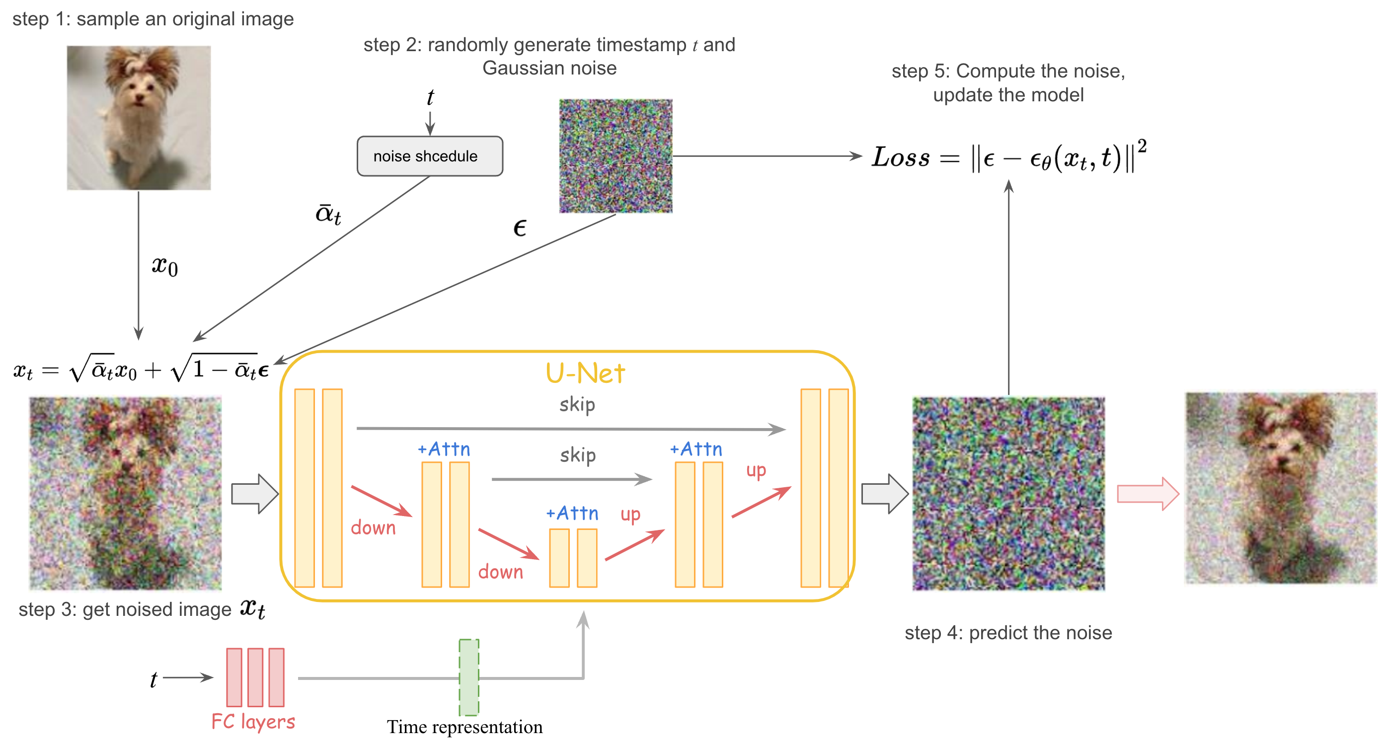
Although the diffusion model involves a lot of mathematics and derivation, its implementation is very concise. The figure below shows the training process of the diffusion model.

The training and sampling algorithms in DDPM can be represented as:

DDPM uses U-Net with residual block and self-attention block as the noise prediction model. Its encoder first down-samples the input to reduce the size of the feature space, and then the decoder restores the feature to the same dimension as the input. The decoder also introduces skip connections to concatenate the features of the same dimension of the encoder. In order to reuse models with different time stamps, time embedding is used to encode timestamp information into the network as the input to each residual block, so that only one shared U-Net is trained.

Improved DDPM [3]

Log-likelihood is important for generative models because it forces the models to capture all the modes of the data distribution. Recent work has shown that small improvements in log-likelihood can have a dramatic impact on sample quality and learned feature representations. However, DDPMs perform poorly on log-likelihood. So this work proposed mainly three improvements to help the diffusion models get lower NLL and higher log-likelihood. (Refer to the slides [4] for more details.)

1. Use a better choice of $\Sigma_{\theta}\left(x_{t}, t\right)$

Although fixing the variance can get good performance, it’s a waste not to use it for training. However, it’s hard for a neural network to predict the variance value directly, because it is just a small point on the number line. So here, the model learns a interpolate vector $v$ to interpolate between the upper and lower bound of the variance.

\[\Sigma_{\theta}\left(x_{t}, t\right)=\exp \left(v \log \beta_{t}+(1-v) \log \tilde{\beta}_{t}\right)\]

The new hybrid objective $L_{\text{hybrid}}$ is constructed because $L_{\text{simple}}$ has no constraint on $\Sigma_{\theta}$. $\lambda=0.001$ is small and the gradient of $\mu_{\theta}$ in $L_{\mathrm{vlb}}$ is stopped so that $L_{\mathrm{vlb}}$ guides $\Sigma_{\theta}$, while $L_{\text{simple}}$ is still the main source of influence over $\mu_{\theta}$.

\[L_{\text {hybrid }}=L_{\text {simple }}+\lambda L_{\mathrm{vlb}}\]

2. Improve the noise schedule

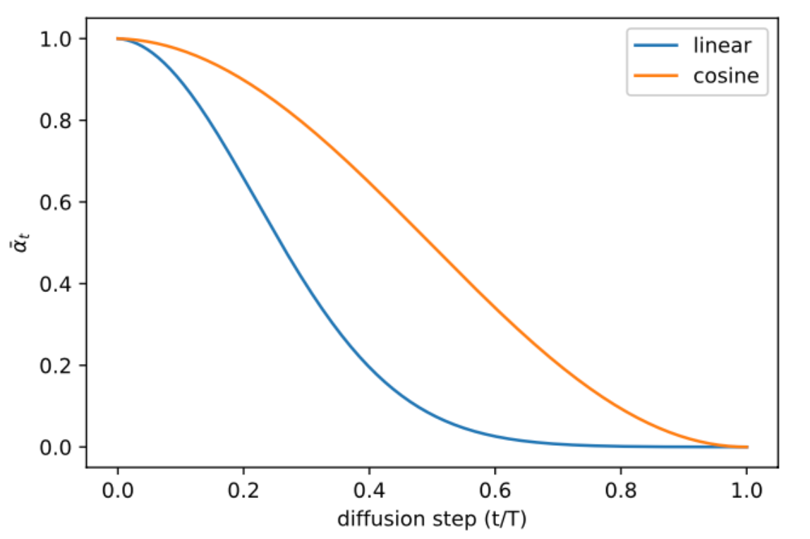
The previous linear noise schedule is sub-optimal for images of lower resolution. The end of the forward noising process is too noisy, and doesn’t contribute very much to sample quality. As shown in the figure, even skipping the 20% reverse process, there is no significant drop in performance. The linear schedule falls towards zero faster, destroying information more quickly than necessary. The authors suggest to use a schedule that has a near-linear drop in the middle, and changes very little near $t = 0$ and $t = T$ to prevent abrupt changes in noise level. The choice of the scheduling function can be arbitrary, and here the cosine schedule is used.

\[\beta_{t}=\operatorname{clip}\left(1-\frac{\bar{\alpha}_{t}}{\bar{\alpha}_{t-1}}, 0.999\right) \quad \bar{\alpha}_{t}=\frac{f(t)}{f(0)}; \quad \text { where } f(t)=\cos \left(\frac{t / T+s}{1+s} \cdot \frac{\pi}{2}\right)\]

3. Reduce gradient noise of loss

Empirically the authors observed that it is pretty challenging to optimize $L_{\mathrm{vlb}}$ due to noisy gradients. Specially, different terms of $L_{\mathrm{vlb}}$ have different magnitudes, and the majority of the loss comes from the first few steps. So they use an important sampling to build a time-averaging smoothed version of $L_{\mathrm{vlb}}$. The learning curves show the efficiency of the proposed method.

\[L_{\mathrm{vlb}}=E_{t \sim p_{t}}\left[\frac{L_{t}}{p_{t}}\right]\]

DDIM [5]

GLIDE

DALLE2

Imagen

GLIDE trains a transformer from scratch using image caption, Imagen takes the off-the-shelf frozen huge language model (T5-XXL), which is more variable. Use UNET for duffusion model, and concatenate it with super resolution diffusion models (same with GLIDE) classifier-free guidance at test time to futher enhance the impact of the text. Generate the image twice (w/ and w/o) the text, calculate their difference, scale it to quite a lot and add it to text-less generation to push it to the direction of text information.

Imagen generate text better than that of GLIDE, but still struggle in compositionality.

How to generate text2image generator more consistently?

Stable Diffusion

Latent Diffusion Models (LDMs)

work on a latent space encoder and decoder (VQGAN? VAE?) are first trained ADV:

• the encoder and decoder can take care of image details and let the diffusion model focus on the important image semantics.
• much faster
• special and suit for art generation because it was trained with LAION-Aesthetics

The main difference is that it adds an encoder and a decoder, because working on the original images (e.g. 512*512) is very expensive. So it uses an auto encoder to first encode the image into a latent space, which will be a lot faster.

Stable diffusion has blown up because it’s free, open-source (for code and weights!) and has good result and has lower computational cost.

Improvements

refer to survey [5]

Diffusion Model for Videos

MAKE-A-VIDEO, IMAGEN VIDEO

References:

[1] What are Diffusion Models?

[2] DDPM: Denoising Diffusion Probabilistic Models

[3] Improved Denoising Diffusion Probabilistic Models

[4] Slides for Improved Denoising Diffusion Probabilistic Models

[5] Denoising Diffusion Implicit Models

another blog should read